Was
Preisendorfer's Rule N used in MBH98 tree ring PC calculations?
Mann
et al. have recently argued that they can salvage MBH98-type results using
correct PC calculations under "the standard selection rule (Preisendorfer's
Rule N) used by MBH98".
http://www.realclimate.org/index.php?p=8
They say that this method permits them to retain 5 PCs in the North American
network. Since the bristlecones are in the PC4, this expanded roster still
permits them to imprint the NH temperature reconstruction. We have discussed
elsewhere many issues regarding the robustness and statistical significance of
this calculation. Here I consider the narrow issue of whether this method was
actually "used by MBH98" for tree ring networks. I have
been able to closely replicate the diagram published at realclimate.org on Nov.
22, 2004, said to be an example of the selection method used in MBH98. I have
tested the 19 network/calculation step combinations used in MBH98 and, in 18 of
19 cases, the selections from the Preisendorfer-type calculation are
inconsistent with the reported selections at the Corrigendum SI. In some cases,
the results are higher; in some cases, lower. In three calculations, different
selections are taken from the same network in different calculation steps - a
result inconsistent with the stated policy. We remain puzzled why Mann et al.
continue to refuse to provide source code for MBH98 calculations and why climate
scientists do not expect them to do so.
Statements
in MBH98
First,
there is no mention in MBH98 or the MBH98 SI that Preisendorfer's Rule N was
used to determine the number of retained PC series for tree ring networks. The
only pertinent reference in MBH98 was as follows:
Certain
densely sampled regional dendroclimatic data sets have been represented in the
network by a smaller number of leading principal components (typically 3–11
depending on the spatial extent and size of the data set). This form of
representation ensures a reasonably homogeneous spatial sampling in the
multiproxy network (112 indicators back to 1820). [our bolds]
This
statement contains no reference to the use of Preisendorfer's Rule N.
In
connection with the calculation of temperature principal component
series, a different calculation, MBH98 does refer to the use of Preisendorfer's
Rule N as follows:
a
conventional Principal Component Analysis (PCA) is performed... An objective
criterion was used to determine the particular set of eigenvectors which should
be used in the calibration as follows. Preisendorfer’s selection rule ‘rule
N’ was applied to the multiproxy network to determine the approximate number Neofs
of significant independent climate patterns that are resolved by the
network, taking into account the spatial correlation within the multiproxy data
set.
Before
trying to interpret these two statements from a text analytic point of view, I
will make four quick points about rules for deciding the number of PCs to
retain:
-
The
briefest survey of PC literature will show that there are many approaches to
selecting the number of PC series to retain and Preisendorfer's Rule N is
far from being a "standard selection rule".
-
in
fact, Urban, in a presentation
about PCs cited on Jan. 6, 2005 by Mann at realclimate
stated that the choice was subjective as follows:
It should be noted that because
the goal of PCA is essentially
utilitarian, the choice of how many axes to retain is ultimately subjective. In
practice, either 2 or 3 axes are retained, simply because it is difficult to
project more than this onto a printed page.
-
Overland
and Preisendorfer [1982] themselves argued that being significant under Rule
N was only necessary for significance; they did not argue that it was
sufficient.
-
The real test for retaining a PC series is not whether it
is significant under Preisendorfer's Rule N (or some other such rule), but whether it is scientifically
significant,. For example, Franklin et al. [1995] stated:
In the final analysis, the
retained
components
must make good scientific sense (Frane & Hill 1976;
Legendre & Legendre 1983; Pielou 1984; Zwick & Velicer 1986; Ludwig
& Reynolds
1988; Palmer 1993).
Now,
from a text analytic perspective, a reasonable reader might conclude that the
difference in description of the PC retention policy in the two cases - tree
rings and temperatures - pointed to the use of different procedures in the two
calculations. In fact, the form of PC calculation in the two calculations
differed: we have determined that the temperature PC calculations were centered
calculations, while, as we've pointed out in our recent articles (and earlier),
the tree ring PC calculations were not conventional centered
calculations. Mann et al. have recently (Jan.
6, 2005) acknowledged that they did not use a "standard centered
method" so their use of an uncentered method is no longer in dispute.
Applying
Preisendorfer's Rule N to Tree Ring Networks
The
real test for whether Preisendorfer's Rule N was used in MBH98 was whether the
actual number of selected PCs can be replicated using this method.
The
actual retentions for each calculation step/network combination were not
provided in MBH98, its SI or at Mann's FTP site. The first complete listing of
actual retentions came in the Corrigendum SI (July 2004). Even the Corrigendum
SI contains no summarized listing: the following table was collated from the
Corrigendum SI and shows the number of retained PCs by calculation step-network
combination. (It was impossible to deduce this table with the additional
disinformation of Mann et al. [2003] that 159 distinct series were used, since
only 139 distinct series were actually used. Any such deduction attempts were
further blocked by erroneous listings of the number of series used in the AD1450
step and the erroneous non-use of 6 available series in the AD1500 step. These
do not affect early 15th century results, but frustrate attempts at
replication.)
|
1400 |
1450 |
1500 |
1600 |
1700 |
1730 |
1750
|
1760
|
1780
|
1800
|
1820
|
| Stahle/OK |
0 |
0 |
0 |
0 |
3 |
3 |
3 |
3 |
3 |
3 |
3 |
| Stahle/SWM |
1 |
1 |
2 |
4 |
7 |
7 |
9 |
9 |
9 |
9 |
9 |
| NOAMER |
2 |
2 |
6 |
7 |
7 |
7 |
9 |
9 |
9 |
9 |
9 |
| SOAMER |
0 |
0 |
0 |
2 |
2 |
2 |
3 |
3 |
3 |
3 |
3 |
| AUSTRAL |
0 |
0 |
0 |
3 |
3 |
3 |
4 |
4 |
4 |
4 |
4 |
| Vaganov |
0 |
1 |
1 |
2 |
2 |
2 |
3 |
3 |
3 |
3 |
3 |
| PC series |
3 |
4 |
9 |
18 |
24 |
24 |
31 |
31 |
31 |
31 |
31 |
| Direct
proxy |
19 |
21 |
19* |
39 |
50 |
55 |
58 |
62 |
66 |
71 |
81 |
| Total
series |
22 |
25* |
28* |
57 |
74 |
79 |
89 |
93 |
97 |
102 |
112 |
Table 1. Proxy series used in MBH98 (collated
from Corrigendum SI, July 2004), showing the number of retained PC series by
network-calculation step combination. *:
The total number of series used in the AD1450 step is incorrectly stated in
MBH98 as 24 (but error is not reported yet). Six series available in the AD1500
network are not used.
The
first hints that a Preisendorfer-type policy had supposedly been used in MBH98
came in our Nature correspondence. In response to our observation of the
error in their PC methods, Mann et al. [Revised Nature Reply] had noticed that, under correct PC
calculations, the bristlecone pine pattern was demoted from the PC1 to the PC4.
precisely the same 'hockey stick'
PC pattern appears using their convention, albeit lower down in the eigenvalue
spectrum (PC#4) (Figure 1a). If the correct 5 PC indicators are used, rather
than incorrectly truncating at 2 PCs (as MM04 have done), a reconstruction
similar to MBH98 is obtained.
They argued that they could still salvage a hockey-stick shaped series using a
Preisendorfer-type calculation on the AD1400 North American network. The
calculation published on Nov. 22, 2004 at realclimate showing the implementation
of a Preisendorfer-type calculation on the AD1400 North American network was
originally submitted in our Nature correspondence. We had seen this diagram and
calculation in August 2004 and had fully considered it in our GRL submission -
in fact, it contributed to the approach taken in our GRL submission, which
differs substantially from our previous Nature submission.
Realclimate Nov 2004 Figure 1
Figure
1 below, http://www.realclimate.org/index.php?p=9
(Nov. 22, 2004), and the two tables are all taken from realclimate, illustrating
the application of the supposed Preisendorfer-type calculation. (The original
section from Preisendorfer is re-typed here for reference.)
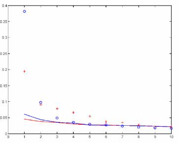
The blue and red lines show the simulation results (using AR1 models of the
AD1400 North American network) under MBH98 and centered PC calculations
respectively; the red and blue points show actual results from the MBH98 and
centered PC methods respectively. Preisendorfer's Rule N selects PC series as
long as the actual eigenvalue exceeds the simulation. For the MBH98 method, 3
eigenvalues are clearly separated under Rule N and perhaps 7 in a centered
calculation. This result is strangely described by Mann et al as follows:
" In the former case, 2 (or perhaps 3) eigenvalues are distinct from the noise eigenvalue continuum. In the latter case, 5 (or perhaps 6) eigenvalues are distinct from the noise eigenvalue
continuum.
It
seems obvious that the selection of 2 (rather than 3) eigenvalues in MBH98
cannot be directly justified on this diagram without appeal to some still
unstated method.
|
 |
| Eigen
# |
%
Variance |
Cum
% Variance |
| 1 |
0.3818 |
0.3818 |
| 2 |
0.0976 |
0.4795 |
| 3 |
0.0491 |
0.5286 |
| 4 |
0.0354 |
0.564 |
| Table 1 (from realclimate - MBH98
method. Bold -retained PCs |
|
| Eigen
# |
%
Variance |
Cum
% Variance |
| 1 |
0.1946 |
0.1946 |
| 2 |
0.0905 |
0.2851 |
| 3 |
0.0783 |
0.3634 |
| 4 |
0.0663 |
0.4297 |
| 5 |
0.0549 |
0.4846 |
| 6 |
0.0373 |
0.5219 |
| Table 2, from realclimate -
centered "MM" method. bold - retained PCs |
|
| FIGURE 1. "Comparison of eigenvalue spectrum resulting from a Principal Components Analysis (PCA) of the 70 North American ITRDB data used by Mann et al (1998) back to AD 1400 based on Mann et al (1998) centering/normalization convention (blue circles) and MM centering/normalization convention (red crosses). Shown also is the null distribution based on Monte Carlo simulations with 70 independent red noise series of the same length and same lag-one autocorrelation structure as the actual ITRDB data using the respective centering and normalization conventions (blue curve for MBH98 convention, red curve for MM convention). In the former case, 2 (or perhaps 3) eigenvalues are distinct from the noise eigenvalue continuum. In the latter case, 5 (or perhaps 6) eigenvalues are distinct from the noise eigenvalue
continuum." Original legend from: Mann, http://www.realclimate.org/index.php?p=9 |
Replication of Realclimate Nov 22, 2004 Figure 1
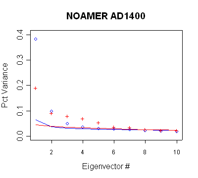
Figure 2 below shows my replication of the above
calculations. The left panel repeats realclimate Nov 22, 2004 Figure 1 (as above), while the right panel shows my emulation, using the script here.
The salient features of the methods are obviously captured.
FIGURE
2.
AD1400 North American network - Preisendorfer-type calculations Left
panel: Mann et al. [realclimate]. Points - NOAMER netowrk; lines -
simulations. Blue - MBH98 decentered; red - centered. Right panel: Emulation
of calculation in left panel.
TESTING OTHER NETWORK/TIMESTEP COMBINATIONS
MBH98 has 6 networks with erratic changes of PC retention by timestep,
yielding a total of 17 network/timestep combinations, all of which are examined
below,
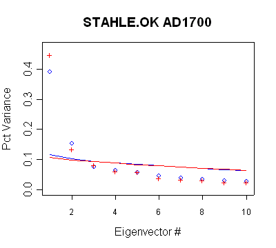
Stahle/OK
MBH98 only used one network/directory combination
here, retaining three PCs. The observed retention is inconsistent with Rule N.
The PC3 is
insignificant under Rule N, but is retained anyway. There is little difference between MBH98 (blue) and
centered (red) results - presumably because Stahle
pre-whitens site chronologies.
 Blue
- MBH98 decentered; red - centered |
|
Eigen #
|
% Var
|
Cum
% Var
|
| 1
|
0.3908
|
0.3908
|
| 2
|
0.1532
|
0.544
|
| 3
|
0.076
|
0.62
|
| 4
|
0.0634
|
0.6834
|
| 5
|
0.0557
|
0.7391
|
| 6
|
0.0463
|
0.7854
|
| MBH98 Eigenvalue Summary.
Blue bold shows retained PCs. The retention of the PC3 is not
consistent with supposed policy. |
|
Stahle/SWM
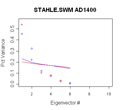
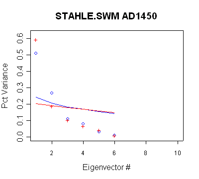
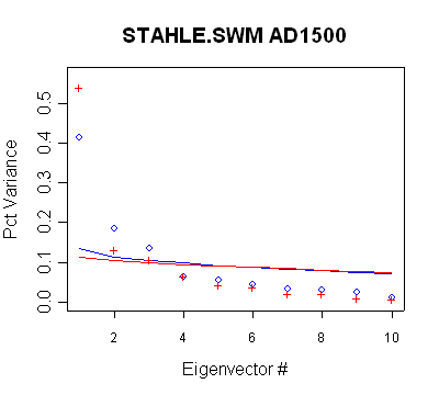
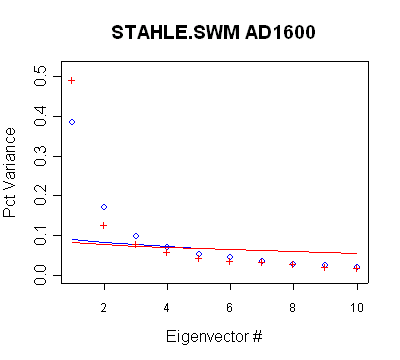
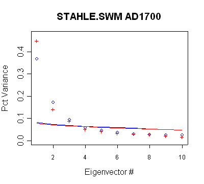
In this network, there are 6 timesteps with different retained PCs. None of
the retention patterns can be obtained through a direct application of Rule N.
- the PC2 in the MBH AD1400 network qualifies under Rule N, but is not used
- the PC2 in the MBH AD1450 network qualifies under Rule N but is not used
- the PC3 in the MBH AD1500 network qualifies under Rule N but is not used
- the PC4 in the MBH AD1600 network does not qualify under Rule N, but is
used anyway;
- the PC4-PC7 in the MBH AD1700 network do not qualify under Rule N, but are
used anyway;
- the PC4-PC9 in the MBH AD1750 network do not qualify under Rule N, but are
used anyway;
- the network does not change between AD1700 and AD1750 and thus Rule N
would not yield a retention change. Nonetheless, two additional PCs are
retained in the AD1750 step.
 Blue
- MBH98 decentered; red - centered |
|
Eigen
# |
%
Variance |
Cum
% Variance |
|
1
|
0.4539
|
0.4539
|
|
2
|
0.3215
|
0.7754
|
|
3
|
0.1187
|
0.8941
|
|
4
|
0.0744
|
0.9685
|
|
5
|
0.0235
|
0.992
|
|
6
|
0.0463
|
0.7854
|
| MBH98 Eigenvalue
Summary. Blue bold shows retained PCs. The non-use of the
PC2 is inconsistent with new policy. (The existence of this
network is inconsistent as well, since there are only 3 sites (6
series) and 2 of the 3 sites appear to be either different
versions of the same site or to contain a splicing error. |
|
 Blue
- MBH98 decentered; red - centered |
|
Eigen
# |
%
Variance |
Cum
% Variance |
|
1
|
0.5072
|
0.5072
|
|
2
|
0.2671
|
0.7743
|
|
3
|
0.1096
|
0.8838
|
|
4
|
0.0783
|
0.9621
|
|
5
|
0.0283
|
0.9904
|
|
6
|
0.0096
|
1
|
| MBH98 Eigenvalue
Summary. Blue bold shows retained PCs. The non-use of the
PC2 is inconsistent with new policy. (The existence of this
network is inconsistent as well, see AD1400). |
|
 Blue
- MBH98 decentered; red - centered. |
|
Eigen
# |
%
Variance |
Cum
% Variance |
| 1 |
0.4134 |
0.4134 |
| 2 |
0.1853 |
0.5986 |
| 3 |
0.1347 |
0.7333 |
| 4 |
0.0627 |
0.796 |
| 5 |
0.0553 |
0.8513 |
| 6 |
0.0437 |
0.895 |
| MBH98 Eigenvalue
Summary. Blue bold shows retained PCs. The non-use of the
PC3 is inconsistent with new policy. |
|
 Blue
- MBH98 decentered; red - centered |
|
Eigen
# |
%
Variance |
Cum
% Variance |
| 1 |
0.385 |
0.385 |
| 2 |
0.1694 |
0.5544 |
| 3 |
0.0972 |
0.6516 |
| 4 |
0.0691 |
0.7206 |
| 5 |
0.0525 |
0.7731 |
| 6 |
0.0441 |
0.8172 |
| MBH98 Eigenvalue
Summary. Blue bold shows retained PCs. The use of the PC4 is
inconsistent with new policy. |
|
 Blue
- MBH98 decentered; red - centered |
|
Eigen
# |
%
Variance |
Cum
% Variance |
| 1 |
0.3683 |
0.3683 |
| 2 |
0.1718 |
0.54 |
| 3 |
0.0945 |
0.6346 |
| 4 |
0.0574 |
0.692 |
| 5 |
0.045 |
0.737 |
| 6 |
0.0365 |
0.7735 |
| 7 |
0.0297 |
0.8032 |
| 8 |
0.0277 |
0.8309 |
| 9 |
0.0247 |
0.8556 |
| 10 |
0.0241 |
0.8797 |
| MBH98 Eigenvalue
Summary. Blue bold shows retained PCs in AD1700 network and
purple bold the additional retained PCs in AD1750 network. The
retention of PC4 and greater is inconsistent with the new policy
as is the increase in the number of PCs in the AD1750 network. |
|
South America
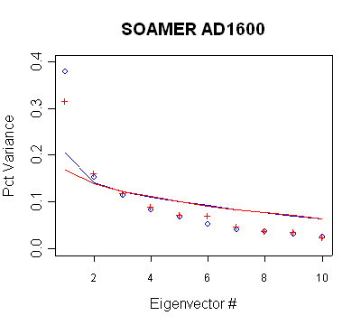
In the South American network, the PC3 is retained for calculation steps after AD1750,
but does not qualify under Rule N. (This network was
also the source of major inconsistencies between the listed sites and the sites
actually used (see Corrigendum), as the network was reduced from 18 sites to 11
sites. The reasons for the inconsistency provided in the Corrigendum are
incorrect, as I'll post on another occasion.)
 |
|
Eigen
# |
%
Variance |
Cum
% Variance |
| 1 |
0.379 |
0.379 |
| 2 |
0.1528 |
0.5318 |
| 3 |
0.1145 |
0.6463 |
| 4 |
0.0832 |
0.7294 |
| 5 |
0.0681 |
0.7975 |
| 6 |
0.0509 |
0.8484 |
| MBH98 Eigenvalue Summary.
Blue bold shows retained PCs in AD1600-1730 calculation steps;
purple bold in AD1750+ calculation step. The retention of the PC3
is inconsistent with the new policy. The addition of a PC to a
network in a later step is also inconsistent with the policy. |
|
Australia/NZ
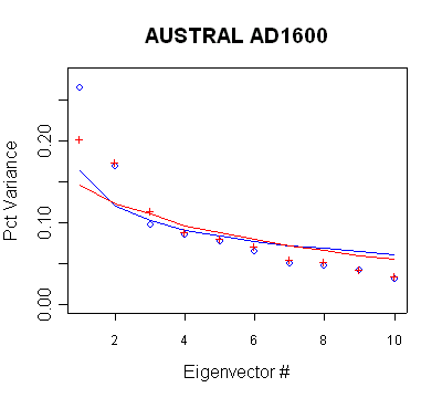
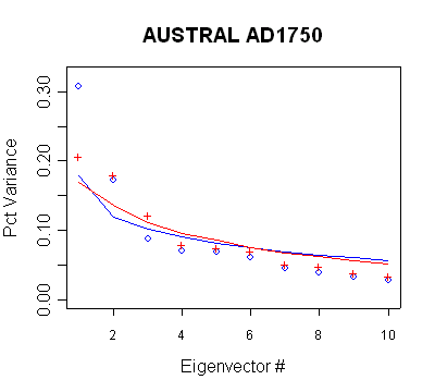
The retention of the PC3 in the AD1600-1730 steps and
the retention of the PC3 and PC4 in the AD1750+ steps is inconsistent with Rule
N.
 |
|
Eigen
# |
%
Variance |
Cum
% Variance |
| 1 |
0.2646 |
0.2646 |
| 2 |
0.1682 |
0.4328 |
| 3 |
0.0974 |
0.5303 |
| 4 |
0.0854 |
0.6156 |
| 5 |
0.0764 |
0.6921 |
| 6 |
0.064 |
0.7561 |
| MBH98 Eigenvalue
Summary. Blue bold shows retained PCs in AD1600-1730
calculation steps. The retention of the PC3 is inconsistent with
the new policy. |
|
 |
|
Eigen
# |
%
Variance |
Cum
% Variance |
| 1 |
0.3074 |
0.3074 |
| 2 |
0.1724 |
0.4798 |
| 3 |
0.0871 |
0.5669 |
| 4 |
0.0702 |
0.6371 |
| 5 |
0.069 |
0.7061 |
| 6 |
0.0611 |
0.7672 |
| 7 |
0.045 |
0.8122 |
| MBH98 Eigenvalue
Summary. Blue bold shows retained PCs in AD1750+ calculation
steps. The retention of the PC3 and PC4 is inconsistent with the
new policy. |
|
Vaganov
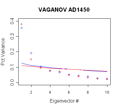
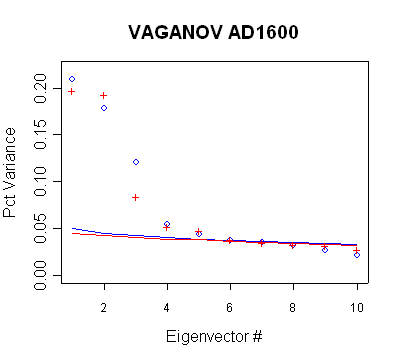
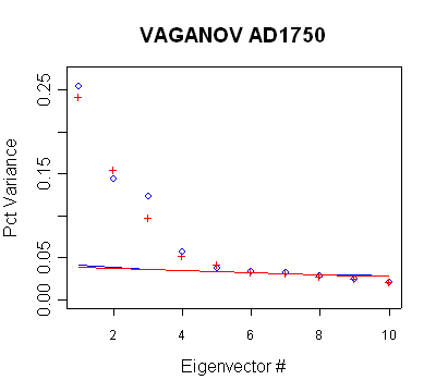
The Vaganov network is a network of Russian sites. There is
relatively little difference between centered and uncentered methods in this
network. This appears to be because of pre-whitening used by Vaganov in
developing tree ring chronologies. The pre-whitening dramatically reduces the
autocorrelation in the network. These graphs are very important in assessing
MBH98 practices, as they show series with large Preisendorfer significance,
which are not used: the PC2 in the AD1450 network, the PC3-5 in all steps from
AD1600 on.
 |
|
Eigen
# |
%
Variance |
Cum
% Variance |
| 1 |
0.3548 |
0.3548 |
| 2 |
0.1914 |
0.5461 |
| 3 |
0.1033 |
0.6494 |
| 4 |
0.0756 |
0.725 |
| 5 |
0.0659 |
0.7909 |
| MBH98 Eigenvalue
Summary. Blue bold shows retained PCs in AD1450-1500
calculation steps. The non-use of the PC2 is inconsistent with
the new policy. |
|
 |
|
Eigen
# |
%
Variance |
Cum
% Variance |
| 1 |
0.2093 |
0.2093 |
| 2 |
0.1782 |
0.3876 |
| 3 |
0.1205 |
0.5081 |
| 4 |
0.0544 |
0.5625 |
| 5 |
0.0433 |
0.6058 |
| MBH98 Eigenvalue
Summary. Blue bold shows retained PCs in AD1600-1730
calculation steps. The non-use of the PC3-PC5 is inconsistent
with the new policy. |
|
 |
|
Eigen
# |
%
Variance |
Cum
% Variance |
| 1 |
0.2541 |
0.2541 |
| 2 |
0.1437 |
0.3977 |
| 3 |
0.1226 |
0.5203 |
| 4 |
0.0562 |
0.5765 |
| 5 |
0.0372 |
0.6137 |
| 6 |
0.0331 |
0.6468 |
| MBH98 Eigenvalue
Summary. Blue bold shows retained PCs in AD1450-1500
calculation steps. The non-use of the PC3-5 is inconsistent with
the new policy. |
|
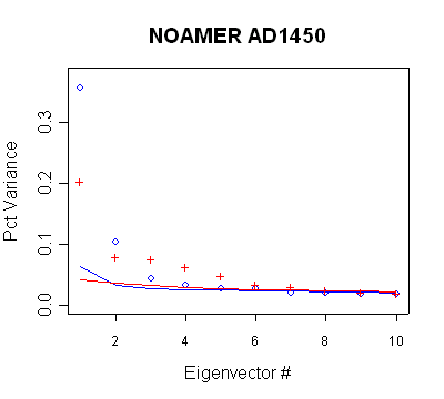
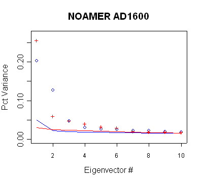
North America after 1400
Again, there are inconsistencies in
the implementation of the supposed policy: a) the non-use of the PC3 and perhaps
PC4 in the AD1450 step; b) the use of the PC5-PC6 in the AD1500 step; c) the
increase in retained PCs (within the same network) from the AD1450 step to the
AD1500 step; d) the non-use of the PC8 in the AD1600 step.
 |
|
Eigen
# |
%
Variance |
Cum
% Variance |
| 1 |
0.3567 |
0.3567 |
| 2 |
0.1032 |
0.46 |
| 3 |
0.0432 |
0.5032 |
| 4 |
0.0319 |
0.5351 |
| 5 |
0.0276 |
0.5626 |
| 6 |
0.0261 |
0.5888 |
| 7 |
0.0203 |
0.609 |
| 8 |
0.0195 |
0.6286 |
| MBH98 Eigenvalue
Summary. This network is used in the AD1450 and AD1500
calculation steps. Blue bold shows retained PCs in the AD1450
calculation step; purple bold the additional PCs retained in the
AD1500 calculation step. The non-use of the PC3-4 is
inconsistent with the new policy, as is the use of the PC5-6 in
the AD1500 step. The change in usage between steps is also
inconsistent. |
|
 |
|
Eigen
# |
%
Variance |
Cum
% Variance |
| 1 |
0.203 |
0.203 |
| 2 |
0.1264 |
0.3294 |
| 3 |
0.0473 |
0.3768 |
| 4 |
0.0295 |
0.4063 |
| 5 |
0.0257 |
0.432 |
| 6 |
0.024 |
0.456 |
| 7 |
0.0223 |
0.4783 |
| 8 |
0.0214 |
0.4996 |
| 9 |
0.0191 |
0.5187 |
| MBH98 Eigenvalue
Summary. Blue bold shows retained PCs in AD1600 calculation
steps. The non-use of the PC8 appears inconsistent with the new
policy. |
|
 |
|
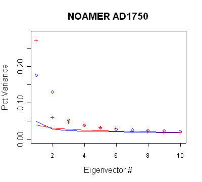
Eigen
# |
%
Variance |
Cum
% Variance |
| 1 |
0.1755 |
0.1755 |
| 2 |
0.1298 |
0.3053 |
| 3 |
0.0509 |
0.3562 |
| 4 |
0.0377 |
0.3939 |
| 5 |
0.0304 |
0.4243 |
| 6 |
0.0266 |
0.4509 |
| 7 |
0.0251 |
0.476 |
| 8 |
0.023 |
0.499 |
| 9 |
0.0215 |
0.5205 |
| 10 |
0.0201 |
0.5406 |
| 11 |
0.0192 |
0.5598 |
| MBH98 Eigenvalue
Summary. Blue bold shows retained PCs in AD1750+ calculation
steps. |
|
Summary
The following table summarizes the inconsistencies between the observed PC
retentions and the retentions according to Rule N. It is obvious that application of the Preisendorfer Rule N method to actual
networks does not yield the PC selections archived at the Corrigendum SI. In
some cases, more PCs are archived; in other cases, fewer PCS: there is no
obvious pattern. In addition, in 3 cases, different selections were made from
the same network, e.g. 7 PCs were selected from the AD1700 SWM network in the
AD1700 calculation; the same network was used in the AD1750 calculation step,
but this time 9 PCs were selected. This would not be permitted without some
still unreported adaptation of the method
| |
Retained PCs |
| Network/Step |
Reported |
Emulated |
| OK/AD1700 |
3 |
2 |
| SWM/AD1400 |
1 |
2 |
| SWM/AD1450 |
1 |
2 |
| SWM/AD1500 |
2 |
3 |
| SWM/AD1600 |
4 |
3 |
| SWM/AD1700 |
7/9 |
3 |
| SOAMER/AD1600 |
2/3 |
2 |
| AUSTRAL/AD1600 |
3 |
2 |
| AUSTRAL/AD1750 |
4 |
2 |
| VAGANOV/AD1450 |
1 |
2 |
| VAGANOV/1D1600 |
2 |
5 |
| VAGANOV/AD1750 |
3 |
5 |
| NOAMER/AD1400 |
2 |
3 |
| NOAMER/AD1450 |
2/6 |
4 |
| NOAMER/AD1600 |
7 |
8 |
| NOAMER/AD1750 |
9 |
10 |
.
Perhaps there is some common factor to the above process that we have not
discerned - however, we are confident that no other third party in the world has
been able to discern the pattern. Had Mann et al. archived their source code for
these calculations (and for other calculations), then these issues would not be
a matter of speculation.
Notwithstanding all of the above, as far as I'm concerned, the main issue is
whether the PC series so selected are significant in a scientific sense,
rather than a data mining sense. We've provided many caveats in our E&E
article to reliance on the bristlecone pine series as arbiters of world
temperature history - whether they are in a PC1 or a PC4. However, if Mann is to
insist at this late stage that the selection of 5 PCs is justified on the
present record, it seems evident to me that an explanation is required for
exactly how the Preisendorfer-policy set forth here can be reconciled with
actual retentions. Perhaps it can, but I've so far been unable to figure out the
secret. These guessing games are also pointless. I invite any readers that have
got this far should express their objections to the U.S. National Science
Foundation and to Nature that this important source code should continue to
remain undisclosed.
References:
Franklin,
Scott B., Gibson, David J., Robertson, Philip A.,Pohlmann, John T. and Fralish,
James S. (1995), Parallel Analysis: a method for determining significant
principal components, Journal of Vegetation Science 6: 99-106.
Overland and Preisendorfer [1982], "A Significance
Test for Principal Components Applied to a Cyclone Climatology", Mon.
Wea. Rev. 110, 1-4.
Footnote: Preisendorfer’s Rule N is a simulation method based on
white noise, stated as follows:
This rule of PC selection is a dominant-variance rule
and is based on a Monte Carlo procedure which simulates sampling from Np(0,Σ),
with Σ=σ2 Ip.
The null hypothesis is that our n x p data
matrix Z has been drawn from such a population. By following the procedure
outlined below, we can systematically accept or reject this hypothesis. Let R be
the centered random data set so formed (cf 5.4 and 5.5). Forming S=RTR
for each such sample, we then build up a cumulative distribution for each of the
ρ = min(n-1,p)) non-zero eigenvalues λj, j = 1,…,ρ.
We can then compare the data eigenvalues of the given n x p data set Z, one by one, with these cumulative distributions. The
details follow.
Construct (say) 100 independent realization of each
of np variates from N(0,1). Form the n x p matrix R as in (5.4) and (5.5). This is the random n x
p counterpart R to the given n x p data matrix Z.
The ωth realization R(ω) of the centered R results in an
ordered sequence of non-zero eigenvalues:
λ1(ω) > …> λρ(ω),
ω = 1, …,100, ρ = min(n-1,p).
Write
Uj(ω) = λj(ω) {
ρ-1 Σk=1:ρ λk(ω)
}–1, ω=1:100, j=1:ρ
For each j, order these (after relabelling) as
Uj(ω1) < …U j
(ω100)
and set
σj(05) = Uj(ω5)
; and σj(95) = Uj(ω95)
;
These σj values define the 5% and 95%
points on the cumulative distribution for the jth random eigenvalues.
For the
given data matrix Z with its associated ordered set of non-zero eigenvalues,
write:
Vj = dj {
ρ-1 Σk=1:ρ dk }-1 j=
1,…ρ
Thus we have
Rule N: p’ is the greatest j for which Vj > σj(95);
0 if no such j exists.
he random n x p counterpart R to the given n x p data matrix Z. The ωth
realization R(ω) of the centered R results in an ordered sequence of non-zero
eigenvalues:
 , ω = 1, …,100, ρ = min(n-1,p).
Write
 ,
ω=1:100, j=1:ρ
For each j, order these (after relabelling) as

and set
 ; and
; and
 ;
;
These σj values define the 5% and 95% points on the cumulative distribution for
the jth random eigenvalues.
For the given data matrix Z with its associated ordered set of non-zero
eigenvalues, write:
 j= 1,…ρ
Thus we have
Rule N: p’ is the greatest j for which Vj > σj(95); 0 if no such j exists.
